Mitscherlich's Law: Generalization with several Fertilizers
H. Schneeberger
Institute of Statistics, University of Erlangen-Nürnberg, Germany
2010, 15thAugust
Abstract
It is shown, that the crop-yield z in dependence on two fertilizers x and y is the product of two components: z in dependence on x alone and z in dependence on y alone, divided by c, the yield without extern fertilizers, i.e. with x = y = 0. For n fertilizers, we have the product of n components, divided by cn-1.
Introduction
If only one fertilizer x is used, the dependence of yield z(x) on x first was given by Mitscherlich (1909) in form of the differential equation
 (1)
(1)
where a is the asymptotic value of z, b the factor of proportionality. As usual in statistics,![]() is the hypothetical value, z the experimental value of the crop-yield. For equation (1) it is assumed: No over-fertilization. For the case of overfertilization see Schneeberger (2009b).
Solution of formula (1) with boundary condition
is the hypothetical value, z the experimental value of the crop-yield. For equation (1) it is assumed: No over-fertilization. For the case of overfertilization see Schneeberger (2009b).
Solution of formula (1) with boundary condition ![]() (x=0) = c is Mitscherlich's curve in the especial instructive form
(x=0) = c is Mitscherlich's curve in the especial instructive form
![]() (2a)
(2a)
demonstrated in figure 1 with c=0.5, a=1.2, b=0,75. For estimation of the parameters in practice see Schneeberger (2009a).
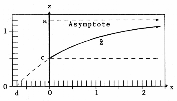
Figure 1:Crop-yield![]() as function of one fertilizer x
as function of one fertilizer x
An other form of formula (2a) is:
![]() (2b)
(2b)
used in the following.
Baule (1918) gave the solution of equation (1) in the form
![]() (3a)
(3a)
with
 (3b)
(3b)
in figure 1 we have d=-0.719.
Generalization
Now we assume two variables (=fertilizers) x and y (see figure 2)
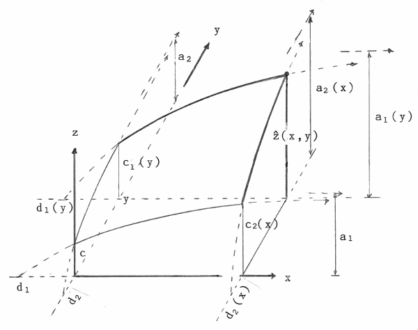
Figure 2:Crop-yield![]() (x,y) as function of two fertilizers x and y
(x,y) as function of two fertilizers x and y
Then we have for the crop-yield![]() (x,y) with formula (2b)
(x,y) with formula (2b)
![]() (4a)
(4a)
and
![]() (4b)
(4b)
Note: For short we write
a1(y = 0) = a1, a2(x = 0) = a2, c1(y = 0) = c2 (x = 0) = c, b1(y = 0) = b1, b2(x = 0) = b2, d1(y = 0) = d1, d2(x = 0) = d2
Generalizing formulae (4) we have
![]() (5a)
(5a)
![]() (5b)
(5b)
and herewith
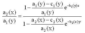 (6)
(6)
Now I make use of a result of Mitscherlich (1947): ..."given different fertilizers, the parameter c (in Mitscherlich's notation) is constant for a fixed fertilizer, as I could prove in tens of years of work"... Mitscherlich's "Wirkungsgrad" c is our parameter b except for the constant ln10. This means:
b1(y) = b1 and b2(x)=b2, indepentent of y resp. x (7)
Herewith we get from formula (6):
 is indepentent of y, i.e.
  (8a)
(8a)
and
 independent of x (8b)
and with this
 independent of y (9a)
and
![]() independent of x (9b)
independent of x (9b)
Finally we have from formula (5a) (or (5b)):
 (10)
(10)
or in the most instructive form
 (11)
(11)
Result: The generalized Mitscherlich formula in two variables is the product of the one-dimensional formulae, multiplied by 1/c.
With formulae (9) one can show, that formula (11) is identical with the formula of Baule (1918).
![]() with
with  (12)
(12)
Equations (10) and (11) can easily be generalized for n fertilizers:
 (13)
(13)
Application
The following data are from an example of Steinhauser, Langbehn and Peters (1992) with x (in 100 kg/ha of P2O5 ), y (in 100 kg/ha of K2O, z (in 1000 kg/ha of rye).
| x1 = 0.25 | x2 = 0.50 | x3 = 0.75 | x4 = 1.00 | x5 = 1.25 | x6 = 1.50 | |
|---|---|---|---|---|---|---|
| y1 = 0.25 | 1.00 | 1.22 | 1.41 | 1.58 | 1.73 | 1.87 |
| y2 = 0.50 | 1.41 | 1.79 | 2.09 | 2.34 | 2.55 | 2.73 |
| y3 = 0.75 | 1.71 | 2.21 | 2.59 | 2.90 | 3.15 | 3.35 |
| y4 = 1.00 | 2.00 | 2.55 | 2.98 | 3.32 | 3.59 | 3.81 |
| y5 = 1.25 | 2.22 | 2.82 | 3.29 | 3.65 | 3.94 | 4.18 |
| y6 = 1.50 | 2.41 | 3.05 | 3.55 | 3.93 | 4.24 | 4.50 |
The 5 parameters were determined with the method of Least Squares of Gauss
 (14)
(14)
summing over all 36 data-points. The minimum was gained iteratively with the non-linear Simplex-Method of Nelder and Mead (1965). The result is
c = 0.2715, a1 = 0.9472, b1 = 0.899, a2 = 1.9438, b2 = 1.027 and
![]()
In figure 3a the contour-lines ![]() (x,y)=0.2, 0.4, ... 4.0 are drawn, in figure 3b intersecting curves
(x,y)=0.2, 0.4, ... 4.0 are drawn, in figure 3b intersecting curves ![]() (x,y = const.) for y=d2, 0, 0.5, 1.0, 1.5 and ∞ are plotted. It is obvious that they are Mitscherlich-curves. We have d1= -0.376, d2 = -0.146. The asymptotes of the curves
(x,y = const.) for y=d2, 0, 0.5, 1.0, 1.5 and ∞ are plotted. It is obvious that they are Mitscherlich-curves. We have d1= -0.376, d2 = -0.146. The asymptotes of the curves![]() (x,y = c) are horizontal dotted straight lines in figure 3b. Especially for y = ∞ we get
(x,y = c) are horizontal dotted straight lines in figure 3b. Especially for y = ∞ we get![]() (∞, ∞)=
(∞, ∞)=![]() = 6.78, Baule's parameter A in formula (12).
= 6.78, Baule's parameter A in formula (12). ![]() (x,y = ∞) is curve a2(x) of figure 2.
(x,y = ∞) is curve a2(x) of figure 2.
In analogy intersecting curves for x=const. could be plotted.
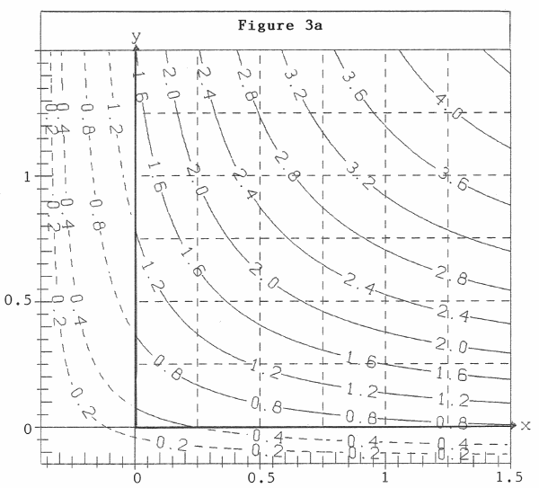
Figure 3a: Contour-lines ![]() (x,y)=const. - in 1000 kg/ha of rye, x in 100 kg/ha of P2O5, y in 100 kg/ha of K2O
(x,y)=const. - in 1000 kg/ha of rye, x in 100 kg/ha of P2O5, y in 100 kg/ha of K2O
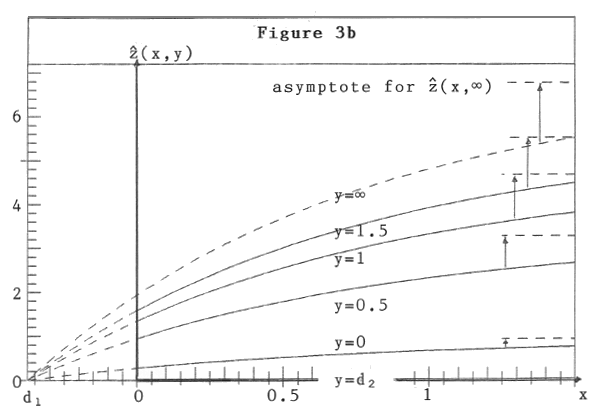
Figure 3b: Mitscherlich-curves ![]() (x,y =const).
(x,y =const).
Example: With fertilizer 100 kg/ha of P2O5 (x = 1) and 50 kg/ha of K2O (y = 0.5) we get the crop-yield 2.335 kg/ha of rye (![]() = 2.335). With x = y = 0 ( i.e. without external fertilizers) we would get 272 kg/ha of rye (
= 2.335). With x = y = 0 ( i.e. without external fertilizers) we would get 272 kg/ha of rye (![]() = c = 0.272)
= c = 0.272)
Acknowledgement
I have to thank Dr. Embacher, Munich, who helped me to publish these papers in the internet.
A generalization with overfertilization is given in paper 5 (Paper 5: Mitscherlich's Law: Generalization with several Fertilizers and Overfertilization)
References
Baule B. (1918). Zu Mitscherlichs Gesetz der physiologischen Beziehungen, Landwirtschaftliche Jahrbücher 51, 363-385
Mitscherlich E.A. (1909). Das Gesetz des Minimums und das Gesetz des abnehmenden Bodenertrags, Landwirtschaftliche Jahrbücher 38, 537-552
Mitscherlich E.A. (1947). Das Ergebnis von über 27000 Feld-Düngungsversuchen, Zeitschrift für Pflanzenernährung, Düngung, Bodenkunde 38. Band, 1947, Verlag Chemie
Nelder J.R. and Mead R. (1965). A Simplex Method for function minimization. The Computer Journal 7, 303-313
Schneeberger H. (2009a). Mitscherlich's Law: Sum of two Exponential Processes. Conclusions. Internet: www.soil-statistic.de, paper 1 and paper 2
Schneeberger H. (2009b). Over-Fertilization: An Inverse Mitscherlich Process. Internet: www.soil-statistic.de, paper 3
Steinhauser H., Langbehn C. and Peters U. (1992). Einführung in die landwirtschaftliche Betriebslehre, Band 1, 5.Auflage