Mitscherlich's Law: A Supplement
Hans Schneeberger
Institute of Statistics, University of Erlangen-Nürnberg, Germany
2010, 1st April
It was shown in Paper 1 (Mitscherlich's Law: Sum of two exponential Processes. Conclusions), that Mitscherlich's curve: crop ŷ in dependence on fertilizer x, can be partitioned into two exponential processes ŷ01 and ŷ02. It will be shown that this partition is indeed of special importance, but it is not the only possible one. There is one further partition of special importance, called here ŷ11 and ŷ12 , and with these two special partitions an infinite number of others is given.
The "experiment", seed and crop, with certain soil, seed, fertilizer etc., as described in Paper 1, in general doesn't result in partition ŷ01 and ŷ02 (this must be corrected), but in one of these infinite partitions. If this one would be known, the loss of soil-immanent fertilizer by the crop and the degree of exploitation of the external fertilizer could be calculated.
Partitions of Mitscherlich's Formula
In Paper 1 already one particular partition of ŷ = ŷ01 + ŷ02 with
 (9)
(9)
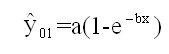
![]() (10)
(10)
is given, see figure 1 and figure 3. ŷ01 is the crop from the external fertilizer, ŷ02 from the soil-immanent fertilizer. ŷ01 is an exponential growing process with asymptote ŷ = a, ŷ02 an exponential declining process with asymptote ŷ =0. So ŷ01 makes most (crop) of the external fertilizer. ŷ02 makes least use of the soil-immanent fertilizer; (9) and (10) is the optimal partition.
The contrary is the case with the partition ŷ = ŷ11 + ŷ12 with
![]() (12a)
(12a)
![]() (12b)
(12b)
see figure 3. Now the crop from the external fertilizer ŷ11 has the asymptote ŷ = a - c, much worse than with ŷ01; ŷ12 = c means, that a maximum of the soil-immanent fertilizer is spent, independent of the quantity of the external fertilizer x. (12a/b) is the poorest partition.
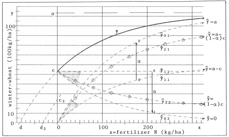
Figure 3: Partition of Mitscherlich's curve ŷ into two components ŷi1 and ŷi2 (i=0,1,2,...)
But with partitions (9), (10) and (12a), (12b) we have an infinite number of further partitions ŷ = ŷ•1 + ŷ•2 ( • for 2, 3, ...):
![]() (13a)
(13a)
![]() (13b)
(13b)
(0 ≤ α ≤ 1)
α = 0 gives the poorest, α = 1 the optimal partition. I will call α parameter of affinity. Because of ŷ•1 = ŷ11 + α(ŷ01 -ŷ11 ) for formula (13a), ŷ•1(x) for fixed x grows from ŷ11(x) to ŷ01(x) with parameter α in a linear way. The same is right with ŷ•2. See the α-scala in figure 3. In addition the curves ŷ•1 = ŷ21 and ŷ•2 = ŷ22 for α = 0.7 are plotted there.
For a special "experiment" a certain value of α will exist. The knowledge of this α would be of great importance for the knowledge of the loss of soil-immanent fertilizer and the effectiveness of the external fertilizer x. The greater α, the better for both results.
If α would be known (e.g. α=0.7, we would have for given x (e.g. 200 kg/ha of N):ŷ22(x) = c2= 24.13(100kg/ha) of winter-wheat, and herewith d2 according to formula (11a) of paper 1: -d2 = 31.65 (kg/ha) of N is the soil-immanent fertilizer, needed for the total crop ŷ(x=200)= 100(100kg/ha) of winter-wheat. In table 2 results for some further values of α are given.
| α | c2 | d2 |
|---|---|---|
| 0 | 53.20 | -83.80 |
| 0.60 | 28.28 | -37.95 |
| 0.65 | 26.20 | -34.76 |
| 0.70 | 24.13 | -31.65 |
| 0.75 | 22.05 | -28.60 |
| 0.80 | 19.98 | -25.63 |
| 1 | 11.67 | -14.36 |
In reversed direction we get α from d2. So the problem of finding α is that of determining the value of d2.
continued 09.01.2012
To demonstrate the dependence of ŷ1 and ŷ2 (in short for ŷ•1 and ŷ•2) on the parameter α, figures 4a, 4b ... 4e give the curves ŷ1, ŷ2 and ŷ = ŷ1 + ŷ2 for α = 0, 0.25, 0.50, 0.75, 1.
Fig. 4a: α = 0; c2 = 53.2, d2 = -83.8
Fig. 4b: α = 0,25; c2 = 42.8, d2 = -62.7
Fig. 4c: α = 0.5; c2 = 32.44, d2 = -44.6
Fig. 4d: α = 0.75; c2 = 22.1, d2 = -28.6
Fig. 4e: α = 1; c2 = 11.7, d2 = -14.4
Fig. 5: α = 0.75; c2 = 32.0, d2 = -43.8
The aim of external fertilization and soil-care must be maximizing ŷ1 and minimising ŷ2, or in short, maximizing α.
How can the value of a fertilizer-soil combination be computed?
With the original data, given in Paper 1, this cannot be done. For that the registration of (at least) one pair of data (x0, d2(x0)), for example for x0=200, is necessary; -d2(x0) > 0 is the quantity of soil-immanent fertilizer, which gives the part of crop ŷ2(x0) = c2(x0). Δ = - d - (-d2(x0)) > 0 is the soil-immanent fertilizer after crop, which can be measured for example with a chemical analysis - as I assume. Herewith we get d2(x0) = d + Δ. Then with d2(x0) the value of c2(x0) - signed in the figures as c2 - is found as solution of
c2 + (a - c2)(1-e-bd2) = 0 or c2 = a(1-ebd2) = ŷ2(x0) (14)
and herewith (see figure 3)
 (15)
(15)
If for example, an experiment with the above soil-fertilizer combination for external fertilizing with x0 = 200 gives the value d2 = -62.7, then the affinity is α = 0.25 (see Fig. 4b). d2 = -28.6 gives α = 0.75 (Fig. 4d). One can see from figures 4b and 4d, that
- The soil-fertilizer combination with higher value of α yields by far the better exploitation of the external fertilizer (see curves ŷ1): for x0 = 200 there is ŷ1(α=0.75)/ŷ1(0.25) = 77.89/57.13 = 1.36; that means, that with the same quantity of external fertilizer x0 = 200 the exploitation is 36 % higher.
- To yield the same total crop ŷ, the part of crop ŷ2 from the soil-immanent fertilizer reduces to about one half in our example: for x0 = 200 we get ŷ2(α = 0.75)/ŷ2(α = 0.25) = c2(α = 0.75)/c2(α = 0.25) = 22.1/42.2 = 0.52. This means: Only 45.6 % of the soil-immanent fertilizer (d2(α = 0.75)/d2(α = 0.25) = 28.6/62.7 = 0.456) is spent in a soil-fertilizer combination with α = 0.75 against one with α = 0.25. The quantity of external fertilizer is the same in both cases: x0 = 200.
I think, this is active soil-conservation.
With n test points (i = 1,...,n) instead of the one x0 we get values α, which are all estimates of the same "true" &alpha (cf. figures 4d and 5 (with x0 = 100)). So our final estimate of α then is Σ α i / n. For gaining the n experimental values αi of course the assumptions of physical experiments must be fulfilled: All experimental parameters are constant, only the value of x is varied. This will be hard to realise in agronomy.
Further interesting questions would arise by changing another parameter, for example the soil, etc.
Acknowledgement
I praise the internet! It gives the possibility to publish works, which are out of the ordinary. I choose this way, after my first paper was returned with the comment "is in its contents fully out of the scope of the journal" (translated from German).