Critique of Mitscherlich's Law in Agronomy II
Supplement
H. Schneeberger
Institute of Statistics, University of Erlangen-Nürnberg, Germany
2018, 13th of March
Introduction
In paper [5] Schneider made an experiment with oats (=z) and three fertilizers nitrogen x1, phosphorus x2 and potash x3. For the reason that z in dependence on each of these fertilizers follows Mitscherlich's law, he concludes, that in his so-called combination-experiment with x2=k2 x1, x3=k3 x1 (k constants) yield z(x1,k2 x1,k3 x1) also grows with x1 according to Mitscherlich's law. At least he makes use of this conclusion.
This conclusion is wrong.
I will show this by a counterexample, and for clearness I will use one with only two fertilizers. In paper [6] - see there in table 1 and also here in table 2 - I used an experiment of Steinhauser et al. with yield z=rye (in 1000kg/ha) and fertilizers x=P2O2 (in 100kg/ha) and y=K2O2 (in 100kg/ha).
In [6] it was shown, that if yield ![]() (x) in dependence on fertilizer x alone follows Mitscherlich's law
(x) in dependence on fertilizer x alone follows Mitscherlich's law
![]() 1(x) = c+(a1-c)(1-e-b1x)=
1(x) = c+(a1-c)(1-e-b1x)= ![]() 1B
1B
and also ![]() 2(y) in dependence on fertilizer y alone follows Mitscherlich's law
2(y) in dependence on fertilizer y alone follows Mitscherlich's law
![]() 2(y) = c+(a2-c)(1-e-b2y) =
2(y) = c+(a2-c)(1-e-b2y) = ![]() 2B
2B
then the two-dimensional yield ![]() B(x,y) is
B(x,y) is
 (12)
(12)
The 5 parameters c, a1, b1, a2, b2 were – as usual – estimated with the method of Least Squares of Gauss, the parameters computed with the nonlinear Simplex-Method of Nelder & Mead [2]. The result is
c=0.2715, a1=0.9472, b1=0.8990, a2=1.9438, b2=1.027
See figures 3a and 3b in [6].
In the present paper in table 2/line 1 the experimental values of yield z are given, in line 3 those of ![]() B according to formula (12). In figure 3b of this paper the figure 3a of [6] is repeated in reduced size. I draw your attention to the good correspondence of experiment and hypothesis in table and figure.
B according to formula (12). In figure 3b of this paper the figure 3a of [6] is repeated in reduced size. I draw your attention to the good correspondence of experiment and hypothesis in table and figure.
| x | 0.25 | 0.5 | 0.75 | 1.00 | 1.25 | 1.50 | line | |
|---|---|---|---|---|---|---|---|---|
| y | ||||||||
| 0.25 | 1.00 | 1.22 | 1.41 | 1.58 | 1.73 | 1.87 | 1 | |
| 1.00 | 1.25 | 1.46 | 1.64 | 1.78 | 1.87 | 2 | ||
| 0.98 | 1.24 | 1.44 | 1.61 | 1.74 | 1.85 | 3 | ||
| 0.50 | 1.41 | 1.79 | 2.09 | 2.34 | 2.55 | 2.73 | 1 | |
| 1.40 | 1.75 | 2.06 | 2.31 | 2.50 | 2.63 | 2 | ||
| 1.42 | 1.79 | 2.09 | 2.33 | 2.53 | 2.68 | 3 | ||
| 0.75 | 1.71 | 2.21 | 2.59 | 2.90 | 3.15 | 3.35 | 1 | |
| 1.76 | 2.20 | 2.58 | 2.89 | 3.13 | 3.30 | 2 | ||
| 1.76 | 2.22 | 2.60 | 2.90 | 3.13 | 3.32 | 3 | ||
| 1.00 | 2.00 | 2.55 | 2.98 | 3.32 | 3.59 | 3.81 | 1 | |
| 2.04 | 2.55 | 2.99 | 3.36 | 3.63 | 3.83 | 2 | ||
| 2.02 | 2.56 | 2.99 | 3.33 | 3.60 | 3.82 | 3 | ||
| 1.25 | 2.22 | 2.82 | 3.29 | 3.65 | 3.94 | 4.18 | 1 | |
| 2.25 | 2.81 | 3.30 | 3.70 | 4.00 | 4.22 | 2 | ||
| 2.22 | 2.81 | 3.29 | 3.67 | 3.97 | 4.21 | 3 | ||
| 1.50 | 2.41 | 3.05 | 3.55 | 3.93 | 4.24 | 4.50 | 1 | |
| 2.38 | 2.98 | 3.50 | 3.92 | 4.24 | 4.47 | 2 | ||
| 2.38 | 3.01 | 3.52 | 3.92 | 4.25 | 4.51 | 3 |
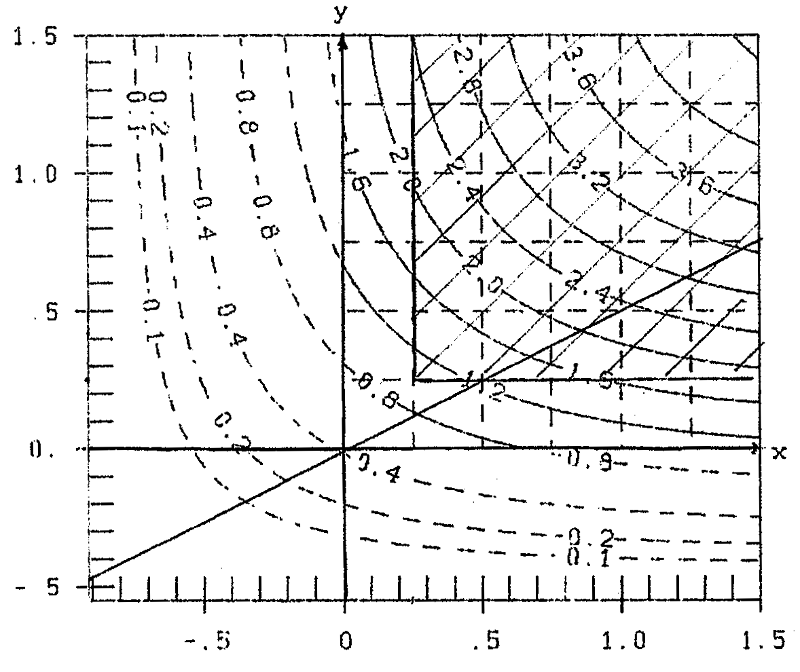
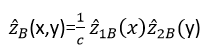
Fig.3a: Contour-lines ![]() A(x,y) for formula (13)
Fig.3b: Contour-lines
A(x,y) for formula (13)
Fig.3b: Contour-lines ![]() B(x,y) for formula (12)
B(x,y) for formula (12)
Now I make my (hypothetical) experiment. I assume, that the fertilizer is a mixture of fertilizers y:x=1:2, or y=0.5x. This line is drawn in figure 3b and in a larger scale in figure 4a. In the side-view in figure 4b you have yield ![]() B in dependence on fertilzer x:
B in dependence on fertilzer x: ![]() B(x,0,5x). This is not a Mitscherlich curve, a curve of decreasing increase with (
B(x,0,5x). This is not a Mitscherlich curve, a curve of decreasing increase with (![]() '>0,
'>0, ![]() ''<0), but a curve of increasing increase with (
''<0), but a curve of increasing increase with (![]() '>0,
'>0, ![]() ''>0).
''>0).
The course of ![]() B (x,0.5x) for larger values of x can be seen in figure 4c/curve B. This curve has a point of inflection at about x=0.25, the value of x, where Steinhauser begins with his experiments. He ends at x=1.5, far enough before overfertilization. See the hatched area in figure 4c. This is the reason for the good correspondence of data and hypothesis in table 2 and figure 3b. B. Schneider in [5] had the luck, that his first experimental value x=0.5 is so great, that it is presumably wide outside the region with (
B (x,0.5x) for larger values of x can be seen in figure 4c/curve B. This curve has a point of inflection at about x=0.25, the value of x, where Steinhauser begins with his experiments. He ends at x=1.5, far enough before overfertilization. See the hatched area in figure 4c. This is the reason for the good correspondence of data and hypothesis in table 2 and figure 3b. B. Schneider in [5] had the luck, that his first experimental value x=0.5 is so great, that it is presumably wide outside the region with (![]() '>0,
'>0,![]() ''>0).
''>0).
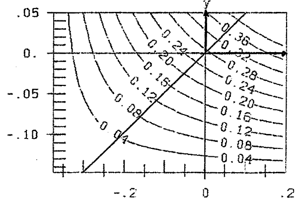
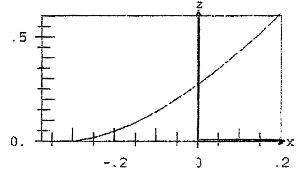
Fig. 4a contour-lines ![]() B (x,y) for formula (12)
B (x,y) for formula (12)
Fig. 4b yield ![]() B along section y=0.5x
B along section y=0.5x
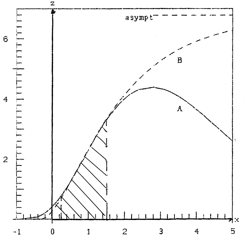
Fig. 4c yield ![]() along the section y=0.5x for hyp. A resp. B
along the section y=0.5x for hyp. A resp. B
Of course I was interested in the question, what would be the consequence, if I would not take Mitscherlich's hypothesis for the depence on the fertiliziers x and y, but my own alternative hypotheses
![]()
Then the consequent generalization for two fertilizers x and y is
![]() 13
13
With the data of Steinhauser the estimation of the 5 parameters A, b1,d1, b2. d2 according to Gauss and Nelder & Mead gives
A=4.741, b1=-0.6629, d1=-0.9146, b2=.0,8079, d2=-0,5506
The yield ![]() A in the data-points (x,y) is given in table 2 (line2) and in figure 3a. You see the good correspondence with the data-values z (in line 1) and with the results according to Mitscherlich
A in the data-points (x,y) is given in table 2 (line2) and in figure 3a. You see the good correspondence with the data-values z (in line 1) and with the results according to Mitscherlich ![]() B (line 3). Correspondingly good ist the correspondence of figures 3a and 3b in the (hatched) area of Steinhauser's experiment.
B (line 3). Correspondingly good ist the correspondence of figures 3a and 3b in the (hatched) area of Steinhauser's experiment.
But this is at an end, when you leave this region, hatched in figures 5a and 5b, i.e when you come near overfertilization. In figure 5a there is a maximum of yield with yield 4.84, while in figure 5b yield extends to a plain with z=6.78, i.e. 40% higher! In figure 5a you can clearly see, that further heightening of yield (beyond the hatched area) requires a disproportional hightening of fertilizing.
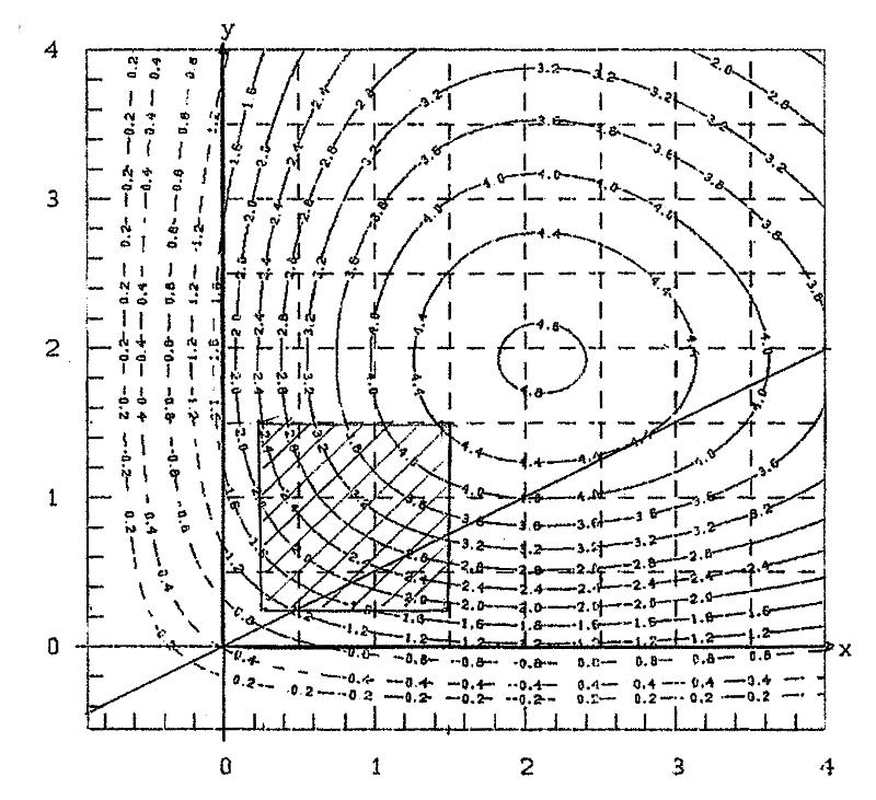
Fig. 5a contour-lines ![]() A, incl. Overfertilization
A, incl. Overfertilization
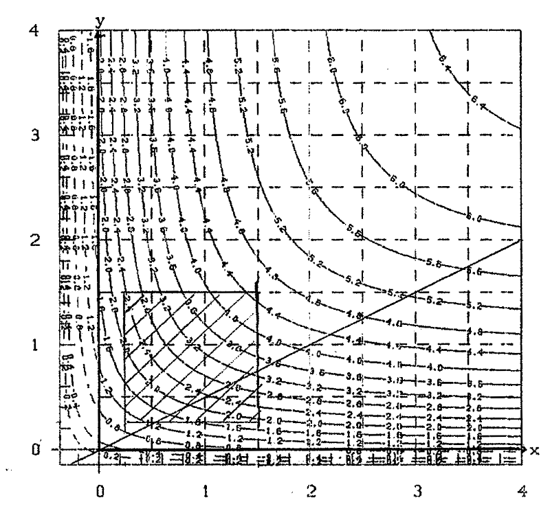
Fig. 5b contour-lines ![]() B, incl. "Overfertilization"
B, incl. "Overfertilization"
In principle it is to say, that the greatest increase of yield is achieved by going vertically to the contour-lines, i.e. along the gradient of ![]() x,y. A different prize of the fertilizers is not considered. As it is in the whole consideration.
x,y. A different prize of the fertilizers is not considered. As it is in the whole consideration.
In figure 4c the yield ![]() A(x,0.5x), i.e. along the section y=0.5x (see figure 5a) is plotted. The maximum of
A(x,0.5x), i.e. along the section y=0.5x (see figure 5a) is plotted. The maximum of ![]() A is 4.4, while the asymptotic maximum of
A is 4.4, while the asymptotic maximum of ![]() B of this section is 6.78, i.e. 54% higher.
B of this section is 6.78, i.e. 54% higher.
References
[1] Mitscherlich, E.A. (1909). Das Gesetz des Minimums und das Gesetz des abnehmenden Bodenertrags, Landwirtschaftliche Jahrbücher, 38, 537-553
[2] Nelder, J.R. and Mead, R. (1965). A Simplex Method for function minimization, The Computer Journal, 7, 303-313
[5] Schneider, B. (1963). Die Bestimmung der Parameter im Ertragsgesetz von E.A. Mitscherlich, Biometrische Zeitschrift, vol.5, issue 2, 78-95
[6] Schneeberger, H. (2010). Mitscherlich's Law: Generalization with several fertilizers. www.soil-statistic.de, paper 4
Download this paper as PDF
Download this Paper in PDF format:
Critique of Mitscherlich's Law in Agronomy II - Supplement [PDF, 1.1 MB]