Critique of Mitscherlich's Law in Agronomy I
H. Schneeberger
Institute of Statistics, University of Erlangen-Nürnberg, Germany
2016, 9th of February
Keywords
power-function, exponential-function, superposition.
Abstract
Hypotheses are presented, which give the yield in dependence on the fertilizer as a growing power-function, superposed (=multiplicated) by an exponential declining function.
Introduction
The problem "dependence of yield on the quantity of fertilizer" seemed to be solved in 1909 with the Law of Mitscherlich [1], the differential equation
![]() = ŷ' = b(a - ŷ) a,b ≥0 (1)
= ŷ' = b(a - ŷ) a,b ≥0 (1)
x = quantity of fertilizer (x ≥ 0)
y = yield (data values); ŷ = hypothetical values
The general solution of (1) is
ŷ = a - (a - ŷ0) e-b(x-x0)
and with the boundary point (x0, ŷ0 =(d,0) we get the special solution
ŷ = a(1-e-b(x-d)) = a(1-e-bz)(2)
The parameters a, b, d are to be estimated.
See figure (1) with the as useful introduced variable z=x-d.
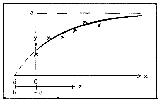
Fig.1: Scheme of Mitscherlich's curve ŷ = a(1-e-bz), z=x-d
Mitscherlich himself was aware of the fact, that for large values of x formula (1) is incorrect [2]. In reality there is no asymptotic constant yield a, but decreasing yield: We have overfertilization. See e.g. [3] .
Because of formula (1) we have ŷ'' = -bŷ' < 0 for z ≥0 and so for the curvature K of ŷ we have
K = 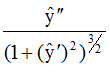 < for z ≥0
i.e. the curve (2) is concave (from below) for z ≥ 0
This was and could be accepted as right up to 1971, as until then no contradictory experiments were known (as far as I know). In 1971 Fox R.L. published the paper "A graphing of corn yield response to added phosphorus on a P-deficient soil (Tropeptic Eurostox)" [4] . Some time ago these results were repeated in the internet and so came to the knowledge of the author. In these papers Fox states "illustration of Mitscherlich's equation of diminishing returns".
These papers do not illustrate Mitscherlich's hypothesis! The curve of yield ŷ (see the curve of Fox and e.g. figure 3) has a point of inflection at x = xW, where ŷ'' = 0 and curvature K = 0.
For x < xW there is ŷ' >0, i.e. K > 0, the curve is convex (from below), the return is not diminishing (as according to Mitscherlich should be), but even growing. For x > xW we have ŷ'' < 0, i.e. K < 0, the curve is convex (from below). Only for x > xW we have ŷ'' < 0. K < 0; the curve ŷ is concave (from below). Only for x >xW the hypothesis of Mitscherlich "diminishing return", is given.
This fact – the visible existence of a point of inflection for x >0 – surely comes from the especially great P-deficiency of the soil in Hawai. It seems, that xW>0 (x = 0 means the beginning of extern fertilization) is a rare case, and that for most soils there is xW < 0 and so the point of inflection doesn't appear in the range of the data, and so cannot be seen.
Hypotheses
Mitscherlich's hypothesis must be corrected in two directions:
- for great values of z there is not an asymptotic constant, but diminishing yield,
- for small values of z there is growing return.
This should be done in one single formula.
Before knowing of Fox' paper, I introduced in a paper [5] , (25th of Sept. 2014) an alternative formula to Mitscherlich's formula (2):
ŷ = aze-bz(3a)
the simplest for term of the family ŷ = azp(E(bz))-1; a, b > 0 (3)
which is the superposition (multiplication) of a power-function zp and the inverse of an exponential function E(bz). The curve of formula (3a) has a maximum at zM = 1/b and one point of inflection at zw = 2/b and is convex (from below) for 0 ≥ z ≥ 2/b . So there is no point of inflection before the maximum, as the result of Fox demands it.: Hypothesis (3a) fulfils direction (1), but not direction (2). See paper [5] , Supplement.
I think, the reader agrees with me, that it is impossible, to give the "right" law: With this single example as data-basis. So I will present a series of hypotheses, which are famous laws in theoretical physics. All are of the simple form (3) with p > 1 and different exponential functions E(bz) – see the used functions (E(z))-1 in figure 2.
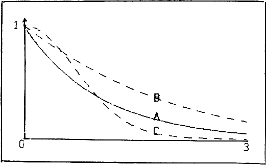
Fig.2: Inverse Exponential Functions
(A) ŷ = (ex)-1; (B) ŷ = ((ex-1)/x)-1; (C) ŷ = (e(x2))-1
H1: The most simple formula of characteristic (3) with p > 1 is ŷ = az2(ebz)-1. So I will work out the results in detail for this case.
H2: ŷ = az3 e-bz (cf. Wien's formula ŷ = z3 e-z (in normed form)).
H3: ![]() (cf. Planck's formula
(cf. Planck's formula ![]() (in normed form)).
(in normed form)).
H4: ŷ = az2(ebz2)-1 = az2e-bz2 (cf. formula of Maxwell-Boltzmann (in normed form)).
For all 4 hypotheses there is ŷ(z = 0) = 0 and ŷ'(z = 0) = 0. So all 4 curves have a convex beginning at z = 0: Direction (2) is satisfied.
Hpyothesis H1: ŷ = az2(ebz)-1 = az2e-bz; z = x-d, a, b > 0 (4)
Unfortunately in Fox' paper no data are given, but only the resulting curve. And I could not get them from the library of the University of Hawai. In addition there isn't a numbered scale on the ordinate of the figure. Nevertheless, to make use of Fox' interesting experiment, I standardised the marks of the ordinate with 1, 2, ... and the values of the abszissa 400, 800,... with 0.4, 0.8, ... (also because of simpler calculation). Results in the original data then can be re-calculated from these results.
As "data" I used – of necessity – the values read from Fox' curve. See table 1.
| x | 0 | .1 | .2 | .3 | .4 | .5 | .6 | .7 | .8 | .9 |
|---|---|---|---|---|---|---|---|---|---|---|
| y | .28 | .48 | .94 | 1.45 | 2.08 | 2.41 | 2.63 | 2.80 | 2.89 | 2.92 |
*In the figures as stars – with the exception of point (x=0,y(0)), which appears as rhombus; this is an excentric of my antique graphic program
With these data I estimated the parameters a, b, d of formula (4) with the method of Least Squares of Gauss and the Method of Nonlinear Optimization of Nelder & Mead [6] ; see also [7] . The result is a=23.61, b=2.09, d=-0.078, therefore
ŷ = 23.61 (x+0.078)2e-2.09(x+0.078)(5)
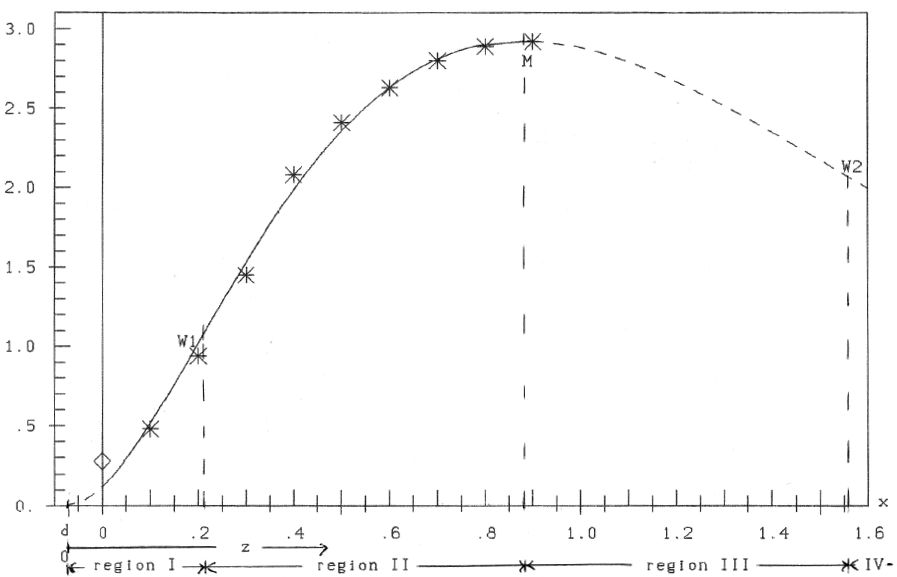
Fig.3: Hypothesis ŷ= az2e-bz; z=x-d
The curve has a maximum (ŷ' = 0) at zM = 2/b = 0.975, xM = zM+ d = 0.88, ŷM = 2.92 and two points of inflection (ŷ'' = 0) at
zW =  : zW1=0.28, xW1=0.202, ŷW1=1.03 and zW2 = 1.633, xW2=1.55, ŷW2=2.074. So we have 4 regions of different character according to table 2:
| Region I | d ≤ x ≤ xW1 | ŷ' ≥ 0 | ŷ'' ≥ 0 |
|---|---|---|---|
| Region II | xW1≤ x ≤ xM | ≥ 0 | ≤ 0 |
| Region III | xM ≤ x ≤ xW2 | ≤ 0 | ≤ 0 |
| Region IV | xW2≤ x ≤ ∞ | ≤ 0 | ≥ 0 |
In region I ŷ is convex (from below), in region II and III concave, in region IV convex. Only in region II one can speak of diminishing return according to Mitscherlich (growing yield ŷ' > 0, but diminishing increase (ŷ'' < 0)).
Hypothesis H1: ŷ = az2e-bz against Mitcherlich's Hypothesis: ŷ = a(1-e-bz)
A. If erroneously all 10 data-points would be used for the computation of the parameters of Mitscherlichs formula (2), the result would be: a=4.025, b=1.596, d=-0.0112; therefore
ŷ = 4.025(1-e-1.596(x+0.0112))(6)
The result in figure 4 demonstrates the bad coincidence of data and computed curve! Quite in contrast to the curve drawn by Fox in his paper.
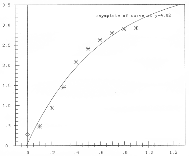
Fig.4: Mitscherlich's curve ŷ = a(1-e-bz), z=x-d, computed with all data
B. If against that only the 8 data with x = 0.2, ...,0.9 ( ≈ region II) are used for computation of the parameters of Mitscherlichs curve, we get: a=3.152, b=3.573, d=+0.107); therefore
ŷ = 3.152(1-e-3.573(x-0.107))(7)
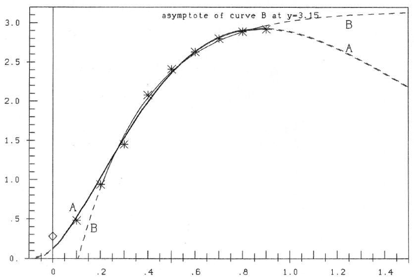
Fig.5: Hypothesis A: ŷ = az2e-bz, z=x-d, computed with all data; against Mitscherlich' hypothesis (B), computed only with data of region II
In figure 5 the curve to formula (7) is shown, and for comparison the curve to formula (5). One can see, that now in region II there is a good correspondence. But to compute the parameters, I first must know what data-points belong to region II. In my paper [5] I per optic estimated the point of inflection from the curve of Fox at x ≈ 0.3 (against x ≈ 0.2 with formula (5)).
But that can be concluded from figure 5: If only data of region II are used for computation, Mitscherlichs hypothesis gives a good estimate.
Hypothesis H2 ŷ = az3e-bz; z=x-d, a,b >0 (8)
Computation yields a=59.28, b=3.013, d=-0.171 and so
ŷ = 59.28(x+0.171)3e-3.013(x+0.171)(9)
In figure 6 this curve together with further ones is plotted. One can see, that in the region of the data-points great coincidence of the curves is given. The difference for x < 0 is small, but for x > 0.9, for overfertilization, begins to increase. So experiments into the region of overfertilization could decide on the "goodness" of the various hypotheses.
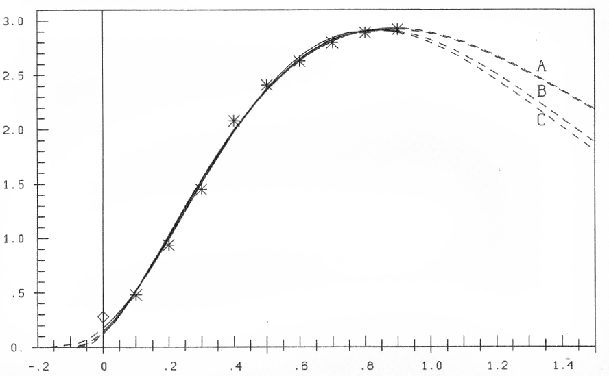
Fig. 6: Hypotheses (A) ŷ = az2e-bz; (B) ŷ = az2![]() ; (C) ŷ = az3e-bz; z=x-d
; (C) ŷ = az3e-bz; z=x-d
Hypothesis H3 ŷ = az2![]() z=x-d; a, b > 0(10)
z=x-d; a, b > 0(10)
We get a=56.06, b=3.012, d=-0.096 and
ŷ = 56.06(x+0.096)2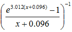 (11)
(11)
The curve also is plotted in figure 6, to show the good coincidence with the other hypotheses in the range of the data-points. So it seems impossible to make a ranking between these 3 hypotheses. The decision could be brought by data in the range of overfertilization. Until then I would prefer hypothesis H1: It is the most simple one of characracteric (3), which fulfils directions (1) and (2)
Until now in the exponential term z only in linear form was presented. That is quite different with the formula of Maxwell-Boltzmann, which I will present at last (accordingly varied).
Hypothesis H4 ŷ = az2(ebz2)-1= az2e-bz2 (12)
Result ŷ = 8.77(x+0.160)2 e-1.104(x+0.160)2 (13)
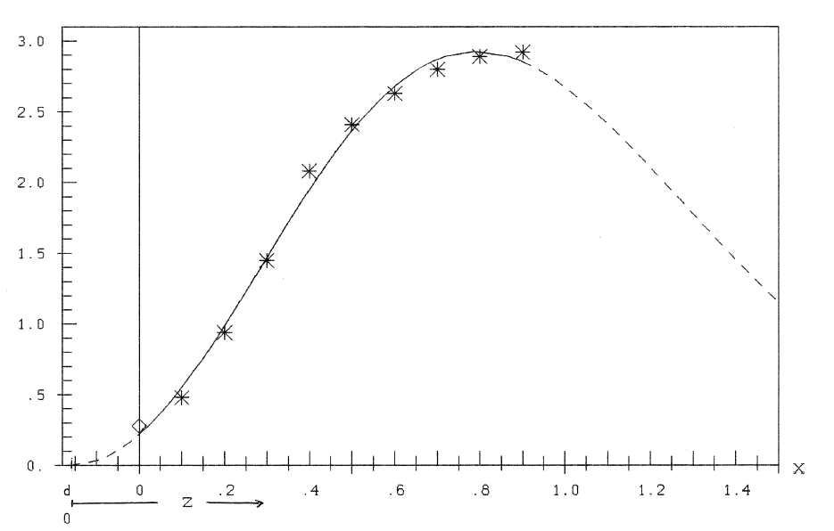
Fig.7: Hypothesis ŷ = az2e-bz2; z=x-d
Summary
Mitscherlich's "Law of diminishing return" is a good hypothesis for the dependence of yield on fertilizer, if one knows the region, where the return is diminishing (ŷ' > 0, ŷ'' < 0). This grave restriction is avoided by the proposed hypotheses: power-functions, superposed by exponentially declining functions. Furthermore the conditions ((ŷ' > 0, ŷ'' > 0) for the region before and correspondingly afterwards (overfertilization) are fulfilled. Further analysis of these hypotheses with highly efficient experiments (pot-experiments ?) would be necessary . As present hypothesis of working I propose the simplest hypothesis (4). A recommendation as a layman: First make the soil nutrient-poor; then begin with fertilizing. For: It's a long way to Hawai!
References
[1] Mitscherlich E.A. (1909). Das Gesetz des Minimums und das Gesetz des abnehmenden Bodenertrags, Landwirtschaftliche Jahrbücher 38, 537-552.
[2] Mitscherlich E.A. (1948). Die Ertragsgesetze, Deutsche Akademische Wissenschaften, Heft 31
[4] Fox, Robert L. (1971) and internet. Growth response curves - The law of diminishing return
[6] Nelder J.R. and Mead R. (1965). A Simplex Method for function minimization, The Computer Journal 7, 303-313
Download this paper as PDF
Download this Paper in PDF format:
Critique of Mitscherlich's Law in Agronomy I [PDF, 667 kB]