Liebig's Law: An Application of Generalized Mitscherlich's Law
H. Schneeberger
Institute of Statistics, University of Erlangen-Nürnberg, Germany
2010, 10th December
Abstract
Liebig's Law and his barrel-model are another presentation of the generalized Law of Mitscherlich. The staves of Liebig are not only of different length, but also with different scales.
Introduction to Liebig's Barrel
The nowadays as Liebig's Law well-known fact originally was found by Carl Sprengel (1828); later popularized by Justus von Liebig (1803-1873). It says that only by increasing the amount of the limiting nutrient the crop-yield can be improved, independent of the other nutrients. The model of this is Liebig's barrel with the fertilizers as staves and the crop-yield as liquid - see the following figure 2.
It was shown in Mitscherlich's Generalized Law (Schneeberger, 2010b, paper 4), that the crop-yield ![]() (x1,.., xn) (
(x1,.., xn) (![]() for the hypothetical, z for the experimental crop-yield) as function of the n fertilizers x1,.., xn is the product of the one-dimensional functions
for the hypothetical, z for the experimental crop-yield) as function of the n fertilizers x1,.., xn is the product of the one-dimensional functions ![]() (0,..xi,..0) multiplied by 1/cn-1, where c is the crop-yield for fertilizers xi=0. This was demonstrated with an example for n=2 in figures 3a and 3b and especially sketched in figure 2 of paper 4.
(0,..xi,..0) multiplied by 1/cn-1, where c is the crop-yield for fertilizers xi=0. This was demonstrated with an example for n=2 in figures 3a and 3b and especially sketched in figure 2 of paper 4.
Deduction of Liebig's Barrel
In figure 1a the essential parts of figures 2 and 3, paper 4, for n=2 fertilizers x1 and x2 are repeated
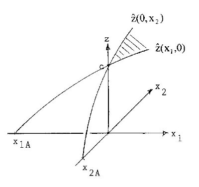
Figure 1a: Mitscherlich's curves ![]() (x1,0) and
(x1,0) and ![]() (0,x2); x1A=-0.376, x2A=-0.146
(0,x2); x1A=-0.376, x2A=-0.146
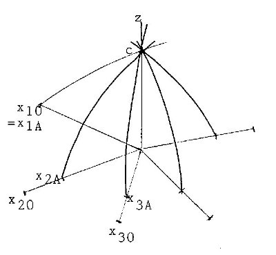
Figure 1b: Generalization of figure 1
-xiA> 0 (i=1,2) are the quantities of fertilizer i, which yield crop ![]() =c, i.e. only with soil-immanent fertilizer. With n fertilizers we use the illustration in figure 1b. In general there will be -xi0 > -xiA >0, where -xi0 is the total quantity of soil-immanent fertilizer i, available in the soil for the experiment.
=c, i.e. only with soil-immanent fertilizer. With n fertilizers we use the illustration in figure 1b. In general there will be -xi0 > -xiA >0, where -xi0 is the total quantity of soil-immanent fertilizer i, available in the soil for the experiment.
Figure 1b already suggests the idea of a cup, turned upside down, where the -xiA >0 are decisive for the contents of the cup. In Liebig's model the xi-axes are broadened to stoves of a barrel of length -xi0>0, the liquid (=crop-yield) c comes up to -xiA ≤ -xi0 of stave i. This means, that the scale is different for different staves. In example of figure 1a the liquid c reaches -xiA=0.376 at stave 1, but -x2A=0.146 at stave 2.
We now assume in figure 1b: x1A=x10, i.e. the whole available fertilizer 1 is spent for the crop. Then the limit of the liquid c is given by the limit of the stave 1 - see figure 2.
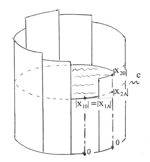
Figure 2: Liebig's barrel
References
Schneeberger, H. (2010b). Mitscherlich's Law: Generalization with several Fertilizers. Internet: http://www.soil-statistic.de, paper 4
Download this paper as PDF
Download this Paper in PDF format:
Liebig's Law: An Application of Generalized Mitscherlich's Law [PDF, 117kB]